GPlates Tutorial: Loading/Saving Data and Changing Colours

1. Author

Kara Matthews¹

¹EarthByte Research Group, School of Geosciences, University of Sydney, Australia

2. Aim

This tutorial is designed to teach the user how to:

Load data
Save data and
Experiment with colours.

Screen shots have been included to illustrate how to complete new steps within each exercise.

3. Included Files

The data bundle for this tutorial, Loading_Saving_Colouring, can be located here. Unarchive the bundle to a folder named Loading_Saving_Colouring, and remember the location so you can access the datasets later. It includes the following GPlates compatible feature files:

See http://www.earthbyte.org/Resources/earthbyte_gplates.html for EarthByte data sets.

4. Background

Feature Collections

Data files loaded into GPlates are referred to as Feature Collections. This is because all data in GPlates are regarded as ‘features’ (e.g. MORs, volcanoes, etc) — whether geological or reconstructed data. For example, the EarthByte Global Coastline File contains the outlines of all the present day coastlines of the world, these coastlines can be thought of as features and therefore when we load the coastline file we are loading a ‘feature collection’. Basins, Cratons, Faults, Hotspots, Isochrons, Mid-Ocean Ridges, Seamounts, Subduction Zones, Sutures and Volcanoes are just some of the other many feature types handled by GPlates. Alternatively a feature can remain ‘unclassified’. Rotation files are also loaded as a Feature Collection.

File Formats

GPlates is able to load and save a number of date-file formats, including PLATES4 line (.dat .pla), GPlates Markup Language (.gpml) and ESRI shape files (.shp). Additionally data can be exported in the GMT xy (*.xy) format.

See the GPlates online manual for further information.

5. Exercise A - Loading Data

In this exercise we will be loading into GPlates the EarthByte Coastline File and the EarthByte Global Spreading Ridge File.

Open GPlates
File → Open Feature Collection… (Figure 1) → locate and select Global_EarthByte_GPlates_Coastlines_20091014.gpml and Global_EarthByte_GPlates_Mid_Ocean_Ridges_20091015.gpml in the Loading_Saving_Colouring data bundle → Open

Note	Hold down the Control (PC) or Command (Mac) key to select multiple files.

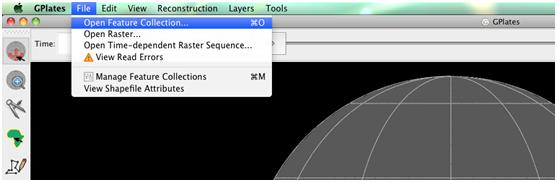
Figure 1: How to load a Feature Collection into GPlates from the menu bar.

The coastlines and spreading ridges of the world are now displayed on the globe.

Using the Drag Globe tool from the Tool Palette spend some time interacting with the globe; rotating it to see the different features. Once you have clicked this icon, click (and hold) anywhere on the globe and drag it by moving the mouse around. While this tool is selected you can drag the globe as many times as you like and rotate it in any direction. You will learn more about controlling the view of the globe in the next tutorial.

The Manage Feature Collections (Figure 2) window is an alternative way to upload data sets. This useful option also enables you to save, unload and switch off data sets. We will make use of the Manage Feature Collections window in Exercise B.

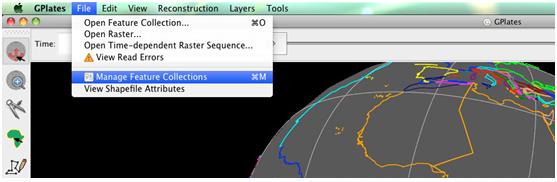
Figure 2: The ‘Manage Feature Collections’ option.

Once data files are loaded into GPlates they can be turned on and off, without being unloaded (ejected). This is a useful, time-saving feature that is especially handy when many different data sets are being viewed and analysed. It can reduce clutter on the globe and help the user to compare data sets without being overwhelmed with too many points, lines or polygons. This functionality is contained within the Manage Feature Collections window.

We will now turn off, and then back on our spreading ridges.

File → Manage Feature Collections → Look under the heading Layer Types (third column of data – Figure 3) and you will notice a small ticked box – by hovering the cursor over this box you will see that it says The file contains feature data in use by GPlates (Figure 4) – now un-check this box (on the line that corresponds to Global_EarthByte_GPlates_Mid_Ocean_Ridges_20091015.gpml) by clicking it (Figure 5).

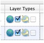
Figure 3: ‘Layer Types’ indicates whether a file is currently in use. In this instance both boxed are ticked, and therefore the feature data are being displayed on the globe.

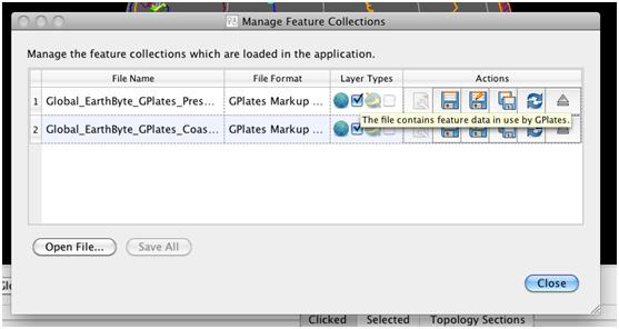
Figure 4: Hovering the cursor over the ticked box provides further information on the status of the relevant data file (in this case the feature data are in use by GPlates).

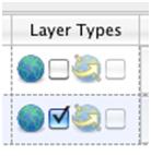
Figure 5: As only one box is now ticked, only one set of feature data is being displayed on the globe.

Now when you look at the globe you will see that the spreading ridge data are no longer displayed. If you go back to your Manage Feature Collections window and hover your cursor over the unchecked box you will see that it now reads The file contains feature data not currently in use by GPlates. Simply re-tick the box and the spreading ridge feature data will appear again!

6. Exercise B - Saving Data Sets

This exercise continues on from the previous exercise. We will now see the different options available for saving data.

Open the Manage Feature Collections window and have a look at the different available actions.
File → Manage Feature Collections (Figures 2 and 6)

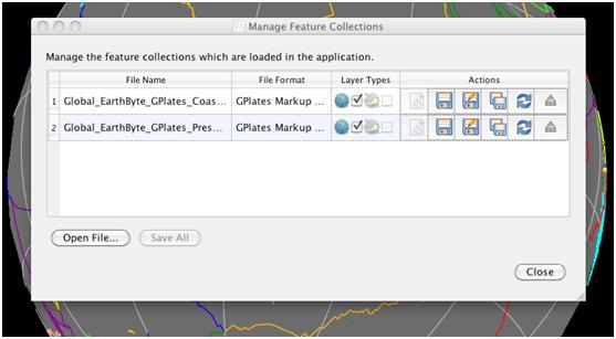
Figure 6: The Manage Feature Collections window.

As you can see, the Manage Feature Collections dialog contains a table of controls and status information about the feature collections that are loaded in GPlates; each row corresponds to a single feature collection, and lists file name, format and available actions. There are three options (‘Actions’) available for saving data:

Save – This first option simply saves the data file using its current name.
Save As – This second option saves the data file using a new name.
Save a Copy – This third option saves a copy of the file using a new name. If this option is selected then the original file will remain loaded in GPlates and the copy will be made in the selected destination.
- In order to practice saving data we will save our coastline file with a new name – EarthByte_Coastlines_Copy (for example). Click the Save As icon and enter the new file details in the Save File As window that appears (Figure 7), leave the file format as GPlates Markup Language (*.gpml).

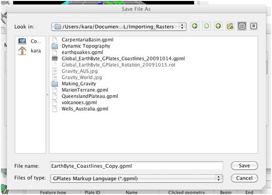
Figure 7: The ‘Save As’ window where a new file name, and optionally a new file format, are specified.

Notice that the File Name in the Manage Feature Collections window has updated itself. You could now work on this file, for example add features to it, and not have to worry about modifying the original contents of the file.

We will leave the current feature collections loaded ready for the next exercise.

7. Exercise C - Changing Feature Colours

In this exercise we will learn how to experiment with feature colours. Features in GPlates can be coloured according to their attributes or they can be assigned a single colour scheme. This functionality improves the user’s ability to effectively view and analyse data, particularly multiple data sets. By default features are coloured by Plate ID. Other colouring options include: Plate ID (by region), Single Colour, Feature Type and Feature Age. Note that you can only change the colour scheme for all features, not individual features.

As a first example we will colour our feature collections using a single colour.

Layers → Geometry Colours → Single Colour → Blue (Figures 8 and 9)

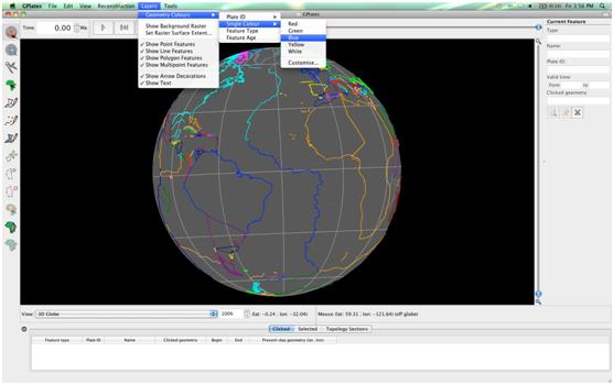
Figure 8: How to experiment with different feature geometry colours using the ‘Geometry Colours’ options in the Layers menu

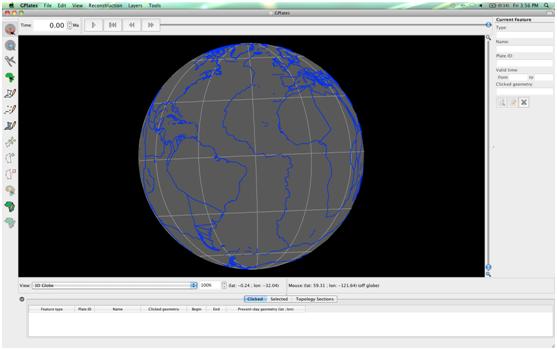
Figure 9: Coastlines and spreading ridges coloured blue.

Now spend some time trying the different colouring options (Figure 10).

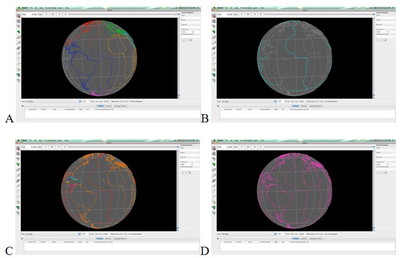
Figure 10: Globe coloured by: A) Plate ID (by region), B) Feature Type, C) Feature Age and D) Single Colour (customised).

To end this exercise we will unload all our data leaving the globe empty. The Manage Feature Collections window (Figure 3) allows us to ‘eject’ data file.

File → Manage Feature Collections → Eject (click this icon for both data sets) → Close

Your globe now appears empty and no data files are loaded into GPlates.