1. Aim
This tutorial, Changing Rotations, separated into two parts, is designed to:
-
Introduce the plate hierarchy and Plate ID’s
-
Rotating features on the globe and
-
Applying and modifying the rotations of an existing plate model
-
Adding a new feature and applying rotation attributes
Part 1 will establish the basics and applying rotations to South America and Africa and will include four exercises: Plate Hierarchy, Rotating features on the globe, Applying a rotation and Modifying an existing rotation.
Part 2 will expand on these concepts with a more advanced exercise looking at SE Asia where we will add a new feature (terrane in Borneo), apply a Plate ID and rotation and will include 4 exercises: Plate hierachy for SE Asia, Importing a new terrane, Rotating new terrane relative to Borneo and an additional exercise.
2. Included Files
For this part of tutorial you will need the data bundle found here. Unarchive the bundle to a folder named GPlates_Rotations_Tutorial, save the datasets above into this folder, and remember the location so you can access the datasets later. The bundle includes the following files:
-
Rotation Model : Africa_SAm_ExampleRotation.rot
-
Coastline File : Africa_SAm_ExampleCoastline.dat
-
Plate ID Table : Global_Earthbyte_PlateIDs_20100211.pdf
Additional datasets and files, including rotations, coastlines, isochrons, spreading ridges and COB files can be downloaded at the following site:
3. Background to Rotations
If you do not have a background in plate motions, we recommend that you read Cox and Hart (1986). Below are some definitions used in this tutorial (see GPlates manual for further details):
A Plate ID assigns a feature to a plate or tectonic element that has moved relatively to other plates for some period during its geological history. A Plate ID is a non-negative integer number.
Tectonic elements can include anything from large plates to island arcs and relatively small blocks or terranes in regions experiencing complex deformation. In GPlates we also assign separate plate IDs to pieces of oceanic crust that were transferred from one plate to another by a ridge jump or propagation. Even though such pieces of crust were always part of one plate or another, we need to assign it a separate plate ID to model this process.
The fixed reference frame of the Earth’s spin axis is assigned plate ID 0, whereas sections of the Earth’s mantle that appear to have moved relatively coherently to other portions of the mantle can be assigned plate IDs as well. For example the Atlantic-Indian hotspots are assigned plate ID 001, whereas Pacific hotspots are assigned plate ID 002. This remains so even for absolute plate motion models that consider relative motion between individual hotspots – however, each mantle plume can ultimately be assigned a plate ID as well, and motion of a given plume relative to the spin axis can be modeled by a set of finite rotations (even though these rotations are not unique). This illustrates that we use plate IDs not only for physical tectonic plates. A list of Plate IDs and corresponding descriptions can be found in the document Global_Earthbyte_PlateIDs_20100211.pdf.
Euler’s Displacement Theorem specifies that any displacement on the surface of the globe can be modelled as a rotation about some axis. This combination of axis and angle is called a finite rotation and can be expressed as a latitude, longitude and angle of rotation. Finite rotations are used by GPlates as the elementary building blocks of plate motion.
Total Reconstruction Poles tie finite rotations to plate motion. A total reconstruction pole is a finite rotation which "reconstructs" a plate from its present day position to its position at some point in time in the past. It is expressed as the combination of a "fixed" Plate ID, a "moving" Plate ID, a point in time and a finite rotation.
Reconstructions are defined in a relative fashion; A single total reconstruction pole defines the motion of one plate id (the "moving" Plate ID) relative to another (the "fixed" Plate ID) at a specific moment in geological time. A sequence of total reconstruction poles is needed in order to fully model the motion of one particular plate across the surface of the globe throughout time.
A sequence of total reconstruction poles is used to model the motion of a single plate across the surface of the globe. Total reconstruction poles describe the relative motion between plates, but ultimately this motion has to be traced back to a single Plate ID which is considered "anchored". GPlates calls this the Anchored Plate ID. Generally, this Plate ID corresponds to an absolute reference frame, such as a hotspot, paleomagnetic, or mantle reference frame. The convention is to assign the anchored Plate ID to 000, but GPlates allows any Plate ID to be used as the anchored Plate ID.
To create the model of global plate rotations that is used in GPlates, total reconstruction poles are arranged to form a hierarchy, or tree-like structure. At the top of the hierarchy is the anchored Plate ID. Successive Plate IDs are further down the chain and linked by total reconstruction poles. To calculate the absolute rotation of a Plate ID of a feature with a given Plate ID (relative to the fixed reference defined by the anchored plate ID, at a given time), GPlates starts at that point in the hierarchy and works its way up to the top - to the root of the tree.
For example, in the GPlates-compatible 2008 EarthByte Global Rotation Model, the South American plate (also known by the abbreviation “SAM”, with plate ID 201) moves relative to the African plate (“AFR”, 701), as does the Antarctic plate (“ANT”, 802), while the Australian plate (“AUS”, 801) moves relative to the Antarctic plate. This is illustrated in Figure 1.
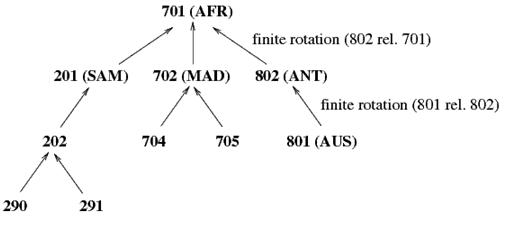
Figure 1: Sample of a simple rotation tree.
Figure 2 is a section from a rotation file. The basic content is the same in other file formats e.g. GPML.
-
Column 1: “Moving” Plate ID e.g. 611
-
Column 2: Time e.g. 0.0 (Ma)
-
Columns 3, 4, 5: Rotation poles. The first two are the coordinates of the pole of rotation (latitude, longitude), the third is the angle of rotation.
-
Column 6: Conjugate or “fixed” Plate ID (Rotations relative to this plate) e.g. 609
-
Column 7: Abbreviation of Plate and Conjugate Plate and name, and sometimes the relevant reference e.g. WPV-NPS West Parece Vela Basin – North Philippine Sea.
There are usually multiple entries for the same Plate ID, but with different times and rotation poles and, sometimes, different conjugate plates, to capture the rotation history of a give plate relative to neighboring, or conjugate plates. Which plate is assigned as a given plate’s conjugate depends on the user. Generally this choice is determined by where most of the constraints for reconstructing the relative motion history are, and this can be time-dependent.
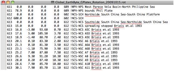
Figure 2: Sample of a rotation file.
4. Exercise A: The Plate Hierarchy
Here we will see what the plate hierarchy looks like in GPlates.
-
Open GPlates
-
Load the rotation file and the coastline file by clicking File → Open Feature Collection, and navigating to the GPlates_Rotations_Tutorial directory.
-
Select the coastline file, Africa_SAm_ExampleCoastline.dat, and the rotation file Africa_SAm_ExampleRotation.rot.
-
Click and drag the globe to rotate it so that it is centered on the South Atlantic. You will see that there are three Plate IDs loaded (each with separate colours) which include the South America, North America and African Plates.
-
We can view the plate hierarchy of the files loaded under Reconstruction → View Total Reconstruction Poles → Reconstruction Tree (third tab). Click Expand All to view the whole tree. You will see that the highest entry id is Plate ID 1 (001 – Atlantic-Indian hotspots) which is fixed to 0 (000 – Earth’s spin axis). The next highest PlateID is 701, which is fixed relative to 001, and in turn, Plates 101 and 201 are fixed to 701.
-
You can try drawing a flow diagram to represent this plate hierarchy.
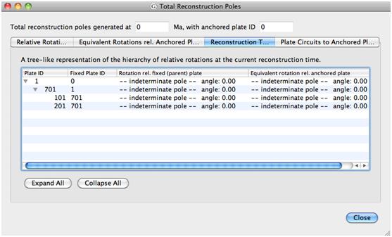
Figure 3: The plate hierarchy tree for our loaded files.
Changing something high in the rotation tree will effect the absolute rotations of all lower plates (relative motions will remain the same). For example, in other datasets you may notice that the South American continent is divided into several plates with different Plate IDs. Rotating (and applying) Plate ID 201 will subsequently move the lower Plate IDs 202, 203… etc, however, if you rotate Plate ID 202, Plate 201 will not be moved as it is higher than 202. You can always check the conjugate plate by looking at the information of a particular plate, or checking the reconstruction tree as above.
5. Exercise B: Rotating Features on the Globe
In this exercise, we will cover the basics on how to rotate a feature on the globe.
In the early 20th century, Alfred Wegener proposed that all continents might once have existed as a single supercontinent. He realised that the coastlines of eastern South America and western Africa fit together like a jig-saw puzzle. Let us start this tutorial by following Wegener’s initial work.
-
With the coastline file, Africa_SAm_ExampleCoastline.dat, and the rotation file Africa_SAm_ExampleRotation.rot already loaded from the last exercise, click and drag the globe to rotate it so that it is centered on the South Atlantic.
|
Note
|
Hold down the Control (PC) or Command (Mac) key to select multiple files. |
-
Our aim is to visually fit South America to Africa. In other words, rotate South America relative to Africa. To select the feature to rotate (South America), click the select feature icon, and then click somewhere on the South American coastline. This will highlight the feature as a white outline. The feature attributes should appear in the panels to the right and bottom of the main reconstruction window. See Figure 4. You will notice that the South American Craton has Plate ID 201. Click on the Africa coastline. What Plate ID corresponds to Africa?
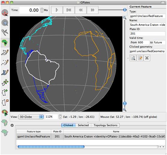
Figure 4: A point along the South American coastline has been selected.
-
Next, click on the Modify Reconstruction Pole
 tool. Note that any other features that have been assigned the same Plate ID will also be highlighted (Figure 5). In this example, the Plate ID of 201 is selected. This is because any changes to a rotation pole for a particular Plate ID will affect all other features assigned to that particular rotation pole. In our case, all the coastlines associated with South America will be highlighted.
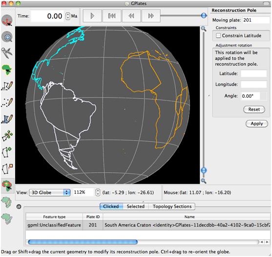
Figure 5: After selecting the Modify Reconstruction Pole, the whole of South America (with the same Plate ID) becomes highlighted.
-
After the feature has been selected by clicking anywhere on the coastline it can be moved anywhere on the globe by dragging. The new location of the plate will be outlined in light grey. See Figure 5. If at first the location you have dragged South America is not correct, just click and drag again as appropriate. The feature can also be rotated about its axis by holding down SHIFT and dragging.
|
Note
|
The globe can still be re-oriented whilst holding down the Command (Mac)/Control(PC) key while in the “Modify Reconstruction Pole” mode. Information regarding the reconstruction pole is displayed in the task panel to the right. This includes the Plate ID of the feature you are moving and the new rotation pole that will be applied if this location is confirmed by pressing Apply (next exercise). |
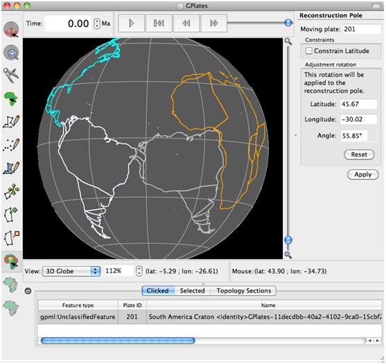
Figure 6: Rotating and re-orienting South America.
6. Exercise B: Applying a Rotation
After you have finished practicing moving a feature, press Reset
 to return South America to its original position. It most likely that for tectonic reconstructions you will be changing the rotation of a feature back in time, rather than changing anything at the present-day. You will notice that by changing the reconstruction time at the top of the window (by sliding the bar, pressing the Rewind
 button or entering a time), none of the features move. This is because the rotation file does not contain any relative rotations. Opening the rotation file in a text viewer, it should appear something like Figure 7. Columns 3, 4 and 5 (the rotation) contain “0.0,” therefore the feature will not move between 0 Ma and 600 Ma. In the next few steps we will apply a reconstruction to South America (Plate ID 201) at 80 Ma.
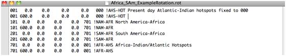
Figure 7: Rotation file
South America started moving westward, separating from Africa, when the South Atlantic Spreading Ridge opened. For the purpose of this exercise lets say that breakup occurred about 80 Ma. We will now apply this to the rotation file.
-
With the rotation and coastline file from Section 1 already loaded, change the reconstruction time at the top to 80 (Ma). As mentioned, none of the features should have moved.
-
As previously mentioned in Section 1, select the Choose Feature
 button, click somewhere on the South American coastline and select the Modify Reconstruction Pole. South America should be highlighted white.
-
Rotate the South American continent back adjacent to Africa (like Figure 6).
-
Once the feature attains the desired position and orientation, clicking Apply will transfer these changes to the rotation file. A new window will pop up asking the user to verify the new relative pole and details (Figure 8). Clicking Ok will change the rotation details of the loaded file.
-
To make these changes permanent you need to save the file in File → Manage Feature Collections; you can Save As
 to a new file or Save
 to overwrite the loaded file.
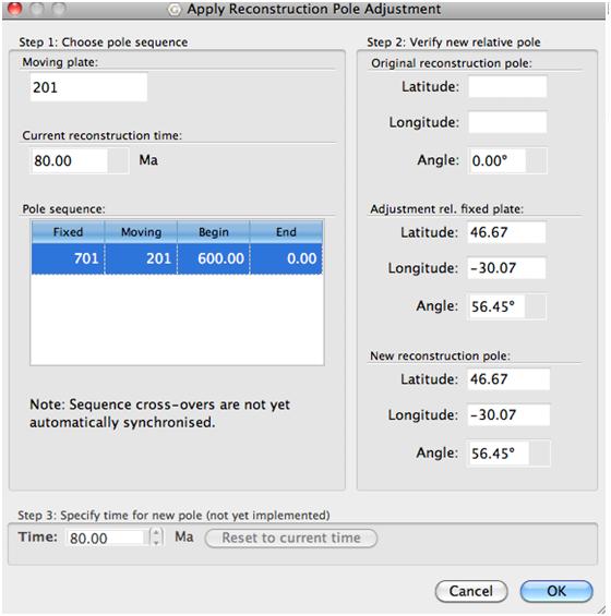
Figure 8: Apply Reconstruction Pole Adjustment window.
-
You can check the new rotation by opening the file and looking at the Plate ID (201). You will see that there is a rotation entry at 80 (Ma) for Plate 201.
-
Now moving forward in time from 80 Ma to present day, South America will move in even increments westward to it’s present day position. By default the original rotation file has 600 (Ma) as the earliest time of rotation, we have not applied a rotation for this time, so between 80 Ma and 600 Ma, South America will rotate back to present day coordinates (0.0 0.0 0.0). This can be rectified by setting your earliest time of rotation to be your earliest reconstruction value (e.g. 80 instead of 600 Ma), populating the rotation entry for 600 Ma by applying a rotation, applying the same rotation (three values) at 600 as 80, or just ignoring what happens prior to 80 Ma.
7. Exercise C: Modifying an Existing Rotation
We now want to apply a second new rotation to South America. For the purpose of this exercise lets say we know that the rate in the first 20 million years of spreading (from 80 Ma to 60 Ma) was much faster than the most recent 60 million years (60 Ma to present day). We have calculated the new location of most eastward point on the coastline of South America to be at approximately lat -8.0 and long -18.0 at 60 Ma.
-
Set the reconstruction time to +60+ (Ma)
-
Select and rotate South America so that the most eastward point on the coastline corresponds to lat -8.0 and long -18.0. You can check this by the looking at the location of the cursor, which will be shown below the window at Mouse: (lat: # ; long #). (See Figure 8)
-
Once the location has been adjusted click Apply and adjust the new rotation pole as listed in Section 1. Remember to save to make the new rotation permanent.
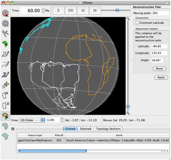
Figure 9: Applying a new rotation to South America at 60 Ma
Now running forward in time, you will see a marked change in the westward translation of South America between 80 Ma to 60 Ma and 60 Ma to 0Ma. Opening the saved rotation file, you will see an entry at 80 and 60 (Ma) for the South American Plate (201), see below. This new addition effectively changes the relative rotation between South America and Africa between 80Ma and 60Ma, as well as 60Ma and 0Ma.
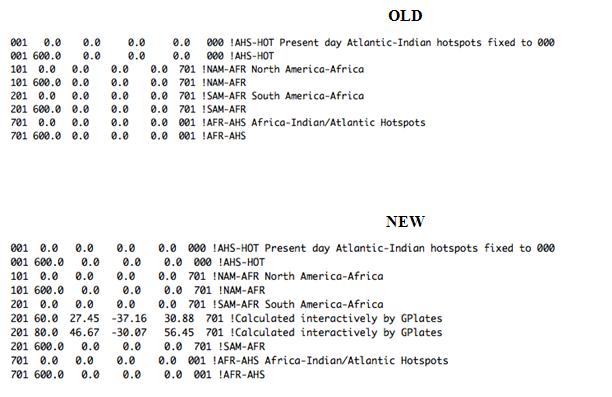
Figure 10: Old and new rotation file.
Note that these subsequent changes will be appended to the loaded file(s), so keep an original if necessary.
The cursor provides longitude and latitude locations to help with re-orienting. This is particularly useful when trying to replicate work from other literature.
Check the existing rotation file for the time increments for the plates. By reconstructing at these times will avoid jumps between two time steps. For example if the existing rotation file has rotations at 10 Ma and 20 Ma, by creating a new rotation at 16 Ma will only change the rotation between 10 Ma and 16 Ma. Between 16 Ma and 20 Ma the plate may jump erratically according to the old pole of rotation, unless you change it or an older timestep.
8. References
Cox, A. and Hart, R.B., 1986. Plate Tectonics: How it Works, Blackwell Scientific Publications, Oxford 392 pp .