1. Aim
This tutorial is designed to teach the user how to manipulate the view of the globe. Screen shots have been included to illustrate how to complete new steps within each exercise.
2. Included Files
The data bundle for this tutorial, Controlling_the_View, can be located here. It includes the following GPlates compatible feature file:
Unarchive the data bundle to a folder named Controlling_the_View, and remember the location so you can access the datasets later.
See http://www.earthbyte.org/Resources/earthbyte_gplates.html for EarthByte data sets.
3. Background
Manipulating the view of the globe enhances the user’s ability to visualise and spatially analyse data sets. GPlates enables the user to rotate the globe in any direction through a fully 360°. Additionally, GPlates supports the Rectangular, Mercator, Mollweide and Robinson map projections.
See the GPlates online manual for further information: http://www.gplates.org/user-manual/Controlling_View.html
4. Exercise A: Manipulating the Globe
In this exercise we will be rotating the globe using the mouse and keyboard.
-
Open GPlates
When GPlates is first opened a grey empty globe appears in the main window with the 0° Meridian running vertically through the centre of the globe (Figure 1A). Even before any data sets are loaded the globe can be rotated. Let’s have a go at moving the globe around using the Drag Globe option
 from the Tool Palette (Figure 1B).
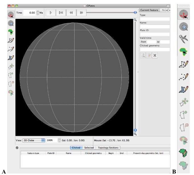
Figure 1: The Main Window (A) – this is how the main window appears when GPlates is first opened, and the Tool Palette that borders the left side of the globe (B) – a collection of tools used to interact with the globe.
-
Click the Drag Globe icon
. Click and drag the globe – i.e. click anywhere on the globe and while holding the mouse button down move the cursor about.
You will notice that the globe moves around with the mouse, in any direction. Whilst the Drag Globe icon is selected you can rotate the globe as many times as you like. Alternatively, while the Drag Globe tool is selected you can move the globe around using the up-, down-, left- and right-keys instead of the mouse. Let’s load some feature data and rotate the globe again.
-
File → Open Feature Collection… (Figure 2) → locate and select Global_EarthByte_GPlates_Coastlines_20091014.gpml from the Controlling_the_View data bundle → Open
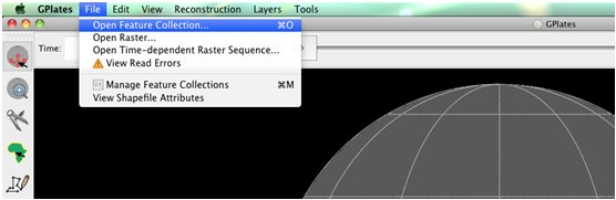
Figure 2: How to load a Feature Collection into GPlates from the Menu Bar.
To practice using the Drag Globe option: (1) rotate the globe so that Antarctica is centre screen (Figure 3), and (2) see if you can use the mouse or the keyboard to position the globe so that Australia is upside down – i.e. at the top of the world (Figure 4).
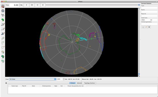
Figure 3. Polar view of the globe centred on Antarctica, achieved using the ‘Drag Globe’ option from the Tool Palette.
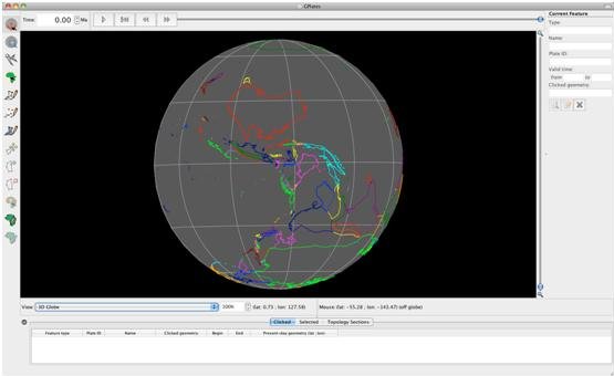
Figure 4. ‘Upside down’ view of Australia, achieved using the ‘Drag Globe’ option from the Tool Palette.
Even if another tool is activated in the Tool Palette the globe can still be re-oriented by holding down the Command (Mac) or Ctrl (PC) key while you click and drag the globe. Let’s practice this by selecting another tool from the Tool Palette and rotating the globe so that Africa appears centered.
5. Exercise B: Camera Control
The camera position (that defines our view of the globe) can also be specified using exact coordinates. In this exercise we will learn how to specify the position of the globe.
-
View → Camera Location → Set Location… (Figure 5)
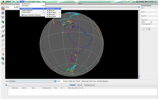
Figure 5. Navigating the Menu Bar to set the camera location.
In the Set Camera Viewpoint window you can specify coordinates where you would like the camera to aim (Figure 6). Let’s aim at Mexico City (Latitude 19.433°; Longitude -99.117°).
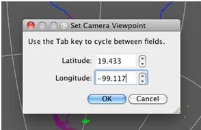
Figure 6. Specifying coordinates to define the camera viewpoint and hence our view of the globe.
-
Now set the camera viewpoint to 48.133° (latitude) and 11.583° (longitude). What continent are we focusing on?
Finally, the globe can be spun around the center viewpoint by holding down the Shift key, and then using the mouse to rotate the globe (have a go at this). You will notice that the globe is turning (pivoting) around this central point in Europe (Munich to be precise).
This feature is also nicely illustrated by first setting the camera projection to 0.00° (latitude), 0.00° (longitude). The rotating globe will look a bit like a pinwheel.
6. Exercise C: Zooming
GPlates enables the user to zoom into regions of interest, or view data at the global scale. There are multiple ways to zoom in and out:
-
the mouse scroll-wheel,
-
the zoom-slider,
-
the Zoom In tool
 (from the Tool Palette),
-
manually entering the zoom level as a percentage (%) using the Zoom Control Field on the main window.
The quickest way to zoom in and out is by using the mouse scroll-wheel, this can be performed regardless of which tool is selected from the Tool Palette.
We will now have a go at zooming into the Hawaiian Islands using the mouse scroll-wheel. But first let’s re-orient the camera viewpoint so that we are focusing on our region of interest.
-
View → Camera Location → Set Location… (Figure 5) → enter the latitude and longitude of Honolulu, Oahu: 21.3°, -157.833° → OK
Now move the scroll-wheel on your mouse backwards and forwards to zoom in and out, respectively. Using a combination of zooming and rotating the globe, zoom into the Big Island (the biggest of the Hawaiian islands) so that it just fits into the screen (Figure 6). Remember that you can hold down the control/command key to move the globe, even if the Drag Globe icon
is not selected from the Tool Palette.
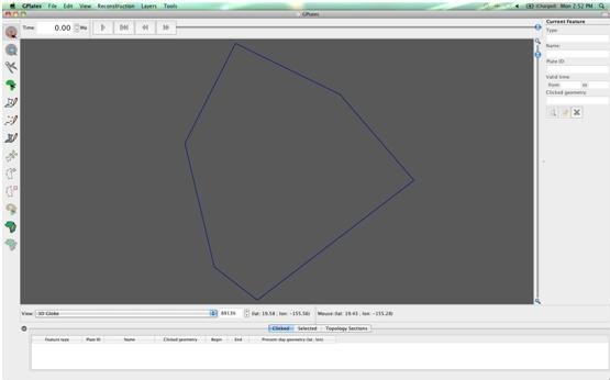
Figure 7. The Big Island, Hawaii.
Now let’s use the Zoom Slider to zoom out again. The Zoom Slider is located on the right side of the main window; it has a magnifying glass with a little ‘+’ symbol at the top of the slider, and a ‘-’ at the bottom. Moving the slider up zooms in and moving it down zooms out. So grab the slider and drag it to the bottom.
By using the Zoom Control Field, located beneath the globe (Figure 8) a percentage of zoom can specified. GPlates allows between 100 – 10000% zoom (100% displays the whole globe in the main window.) The Zoom Control Field can be accessed
-
by directly clicking the text field and typing a number (between 100 and 10000), or
-
from the View option in the Menu Bar.

Figure 8. The Zoom Control Field, located beneath the globe allows the user to specify a percentage of zoom.
Let’s experiment with this second zoom option.
-
View → Camera Zoom → Set Zoom… (Figure 9) → the value in the Zoom Control Field (see Figure 8) will be highlighted, ready for you to replace with a new value, so type a percentage (try 150% so you can see the effect on the globe – Figure 10).
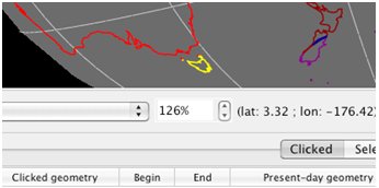
Figure 9. Navigating the Menu Bar to set the camera zoom.
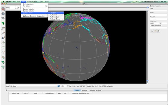
Figure 10. The Hawaiian Islands at 150% zoom (notice that the Zoom Control Field beneath the globe reads ‘150%’).
7. Exercise D: Applying Different Map Projections
GPlates can display data using different map projections (Rectangular, Mercater, Mollweide and Robinson). This allows the user to choose how to best visualise and analyse their data. In this exercise we will practice changing the map projection from the Menu Bar and directly from the main window.
-
View → Set Projection… (Figure 11) → Projection – Mollweide (Figure 12A), Central Meridian 180.00 (Figure 12B) → OK
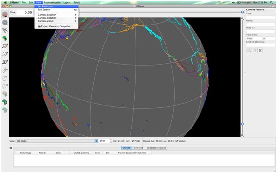
Figure 11. Navigating the Menu Bar to set the map projection.
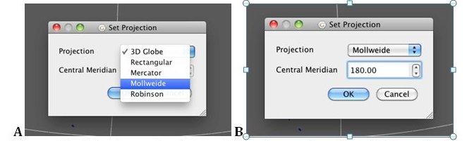
Figure 12. Selecting projection type (A) and central meridian (B) from the ‘Set Projection’ window.
-
Now drag the globe (using the ‘Drag Globe’ tool
) so that the globe is positioned in the middle of the main window (Figure 13).
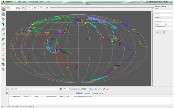
Figure 13. The Mollweide projection centred on the 180° meridian.
Now let’s change the projection again, but this time from the main window. Beneath the globe there is a drop down box entitled View, this contains all the different map projections (Figure 14). Spend some time experimenting with the different options.
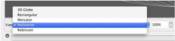
Figure 14. The View dropdown box enables the user to switch between projections from the main window.
To end the exercise change the projection back to 3D Globe.